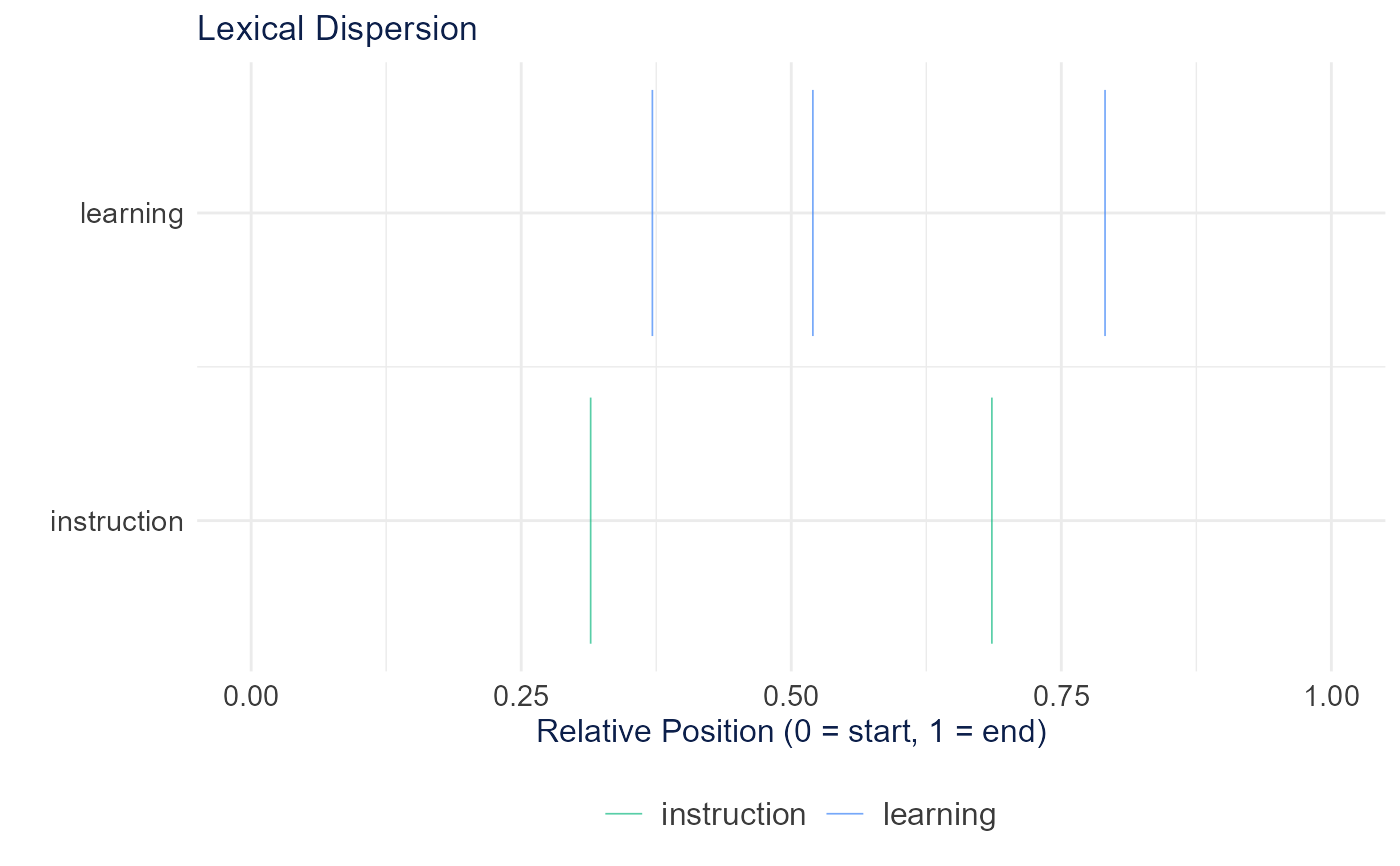
Creates an X-ray plot showing where terms appear across documents. Each row represents a term, and marks indicate occurrences.
Usage
plot_lexical_dispersion(
  dispersion_data,
  scale = "relative",
  title = "Lexical Dispersion",
  colors = NULL,
  height = 400,
  width = NULL,
  marker_size = 8
)
Arguments
- dispersion_data
Data frame from calculate_lexical_dispersion()
- scale
Character, "relative" or "absolute" (must match calculation)
- title
Plot title (default: "Lexical Dispersion")
- colors
Named vector of colors for each term, or NULL for auto
- height
Plot height in pixels (default: 400)
- width
Plot width in pixels (default: NULL for auto)
- marker_size
Size of position markers (default: 8)
Examples
# \donttest{
tokens <- quanteda::tokens(TextAnalysisR::SpecialEduTech$abstract[1:5])
dispersion <- calculate_lexical_dispersion(tokens, c("learning", "instruction"))
plot_lexical_dispersion(dispersion)

# }
# }