Semantic analysis examines relationships of meaning between words and documents. The sections below follow the Shiny app’s Semantic Analysis tabs in order.
Setup
A 150-document subset of SpecialEduTech keeps the build
fast; the full dataset works the same way.
library(TextAnalysisR)

mydata <- SpecialEduTech[1:150, ]
united_tbl <- unite_cols(mydata, listed_vars = c("title", "keyword", "abstract"))
tokens <- prep_texts(united_tbl, text_field = "united_texts", remove_stopwords = TRUE)
dfm_object <- quanteda::dfm(tokens)
Word Co-occurrence
word_co_occurrence_network() builds a network of words
that co-occur across documents, with community detection and centrality
metrics. Edges weight by raw counts; edge_metric = "pmi"
corrects the bias toward generic frequent words.
network <- word_co_occurrence_network(
  dfm_object,
  co_occur_n = 50,
  top_node_n = 30,
  node_label_size = 22,
  community_method = "leiden"
)

network$plot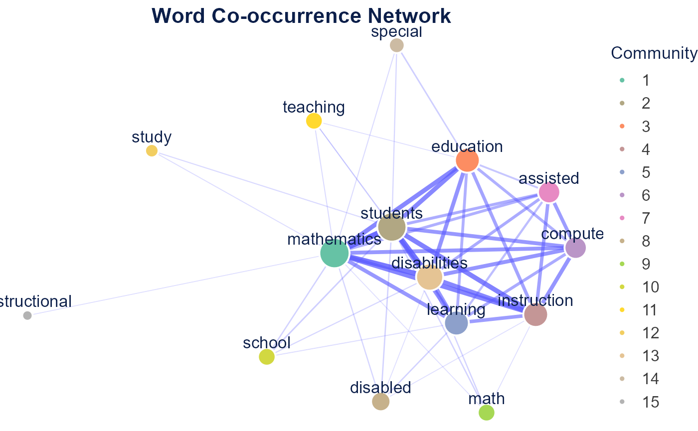
network$tableNetwork Centrality Table
network$summaryNetwork Summary
Word Correlation
word_correlation_network() connects words by phi
correlation of their document co-occurrence patterns.
corr_network <- word_correlation_network(
  dfm_object,
  common_term_n = 15,
  corr_n = 0.3,
  community_method = "leiden"
)

corr_network$plot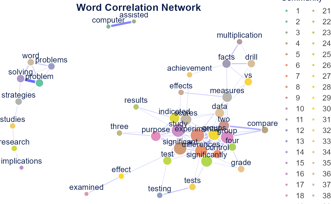
corr_network$tableNetwork Centrality Table
Document Similarity
semantic_similarity_analysis() compares documents by
words, n-grams, or embeddings (embeddings require Python). The example
below uses word features on a subset and renders a cosine similarity
heatmap.
subset_texts <- united_tbl$united_texts[1:10]

similarity <- semantic_similarity_analysis(
  subset_texts,
  document_feature_type = "words",
  similarity_method = "cosine",
  verbose = FALSE
)

plot_similarity_heatmap(similarity$similarity_matrix, method_name = "Cosine")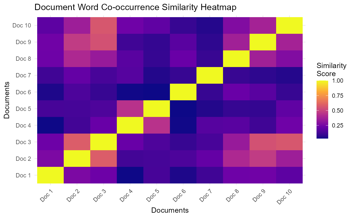
| Method | Description | Requires |
|---|---|---|
| Words | Word-frequency vectors (bag-of-words) | none |
| N-grams | Word-sequence vectors | none |
| Embeddings | Transformer sentence vectors | Python |
Comparative Analysis
Comparative analysis scores how similar documents in one category are
to a reference category.
extract_cross_category_similarities() pulls cross-category
pairs from a similarity matrix and
analyze_similarity_gaps() summarizes the differences. The
example uses the first 30 documents.
term_matrix <- as.matrix(dfm_object)[1:30, ]
normalized <- term_matrix / sqrt(rowSums(term_matrix^2))
sim_matrix <- normalized %*% t(normalized)

docs_data <- data.frame(
  display_name = paste0("doc", 1:30),
  reference_type = quanteda::docvars(dfm_object, "reference_type")[1:30]
)
dimnames(sim_matrix) <- list(docs_data$display_name, docs_data$display_name)

cross <- extract_cross_category_similarities(
  sim_matrix,
  docs_data,
  reference_category = "journal_article",
  category_var = "reference_type",
  id_var = "display_name"
)

gaps <- analyze_similarity_gaps(cross)
gaps$summary_stats
## # A tibble: 1 × 7
## other_category mean_similarity median_similarity sd_similarity min_similarity
## <fct> <dbl> <dbl> <dbl> <dbl>
## 1 thesis 0.268 0.271 0.14 0.025
## # ℹ 2 more variables: max_similarity <dbl>, n_pairs <int>Semantic Search
run_rag_search() retrieves the documents most relevant
to a query using embedding similarity. It requires an OpenAI or Gemini
API key; see AI Integration.
results <- run_rag_search(
  query = "math intervention for students with disabilities",
  documents = united_tbl$united_texts,
  provider = "openai"
)
Sentiment & Emotion
sentiment_lexicon_analysis() scores documents with the
Bing, AFINN, or NRC lexicon. The Bing example runs below.
sentiment <- sentiment_lexicon_analysis(dfm_object, lexicon = "bing")
plot_sentiment_distribution(sentiment$document_sentiment)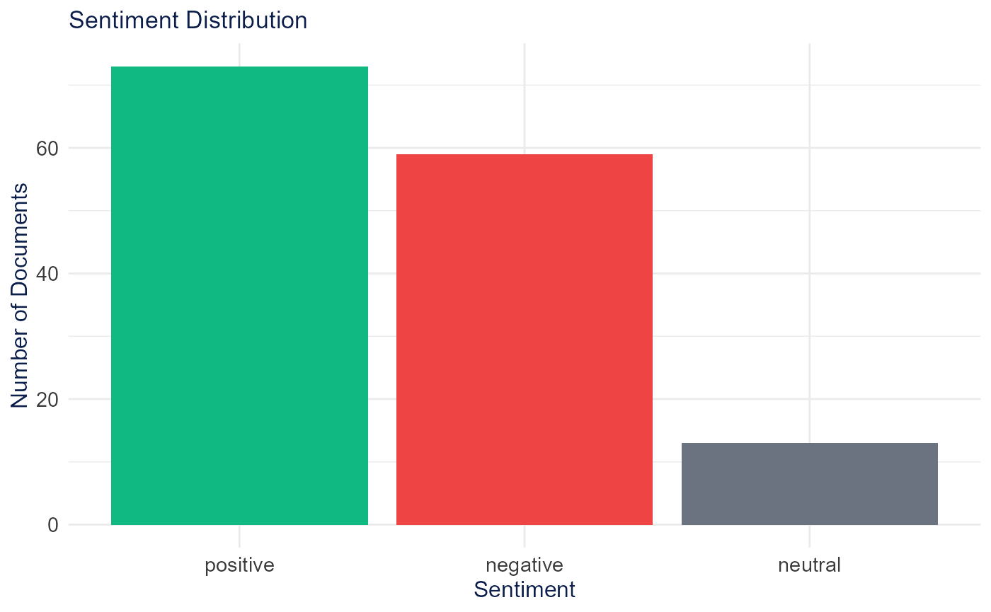
NRC also yields discrete emotions for
plot_emotion_radar(). NRC downloads through
textdata behind a license-gated prompt, so the emotion
example is shown but not run.
emotion <- sentiment_lexicon_analysis(dfm_object, lexicon = "nrc")
plot_emotion_radar(emotion$emotion_scores)
plot_sentiment_by_category() compares sentiment across a
metadata category after joining it to the scored documents. Transformer
(sentiment_embedding_analysis()) and LLM
(analyze_sentiment_llm()) scoring require Python or an API
key and are not run here.
scored <- sentiment_lexicon_analysis(dfm_object, lexicon = "bing")$document_sentiment
scored$reference_type <- quanteda::docvars(dfm_object, "reference_type")[
  match(scored$document, quanteda::docnames(dfm_object))
]
plot_sentiment_by_category(scored, category_var = "reference_type")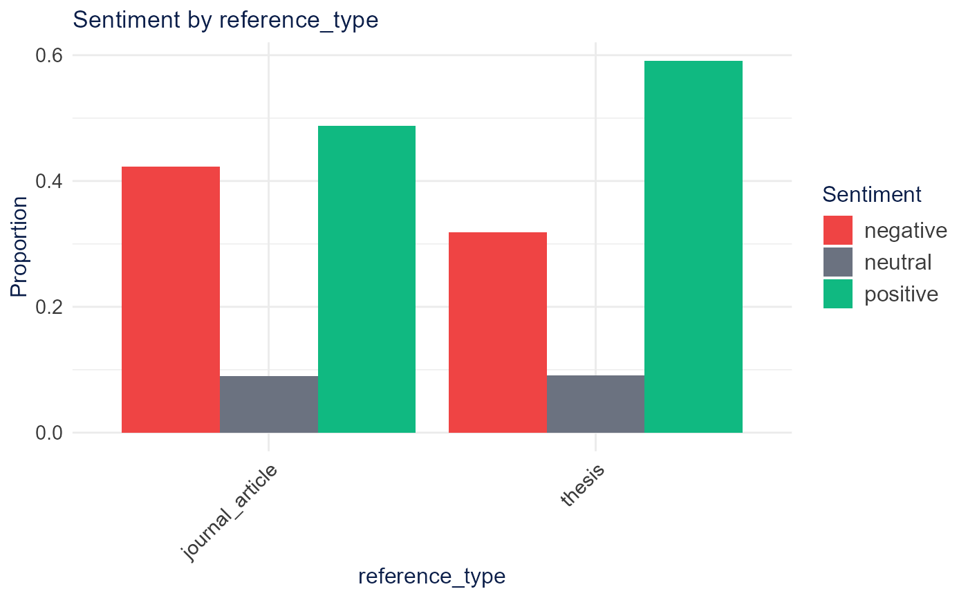
Document Groups
cluster_embeddings() groups documents from a feature
matrix. K-means and hierarchical clustering run in base R; the app’s
default UMAP + DBSCAN path requires Python.
generate_cluster_labels_auto() labels each group with its
most distinctive terms.
data_matrix <- as.matrix(dfm_object)

groups <- cluster_embeddings(data_matrix, method = "kmeans", n_clusters = 5, verbose = FALSE)
groups$n_clusters
## [1] 5
labels <- generate_cluster_labels_auto(data_matrix, groups$clusters, method = "tfidf", n_terms = 3)
labels
## $`1`
## [1] "tutor, reward, arousal"
##
## $`2`
## [1] "educable, mentally, handicapped"
##
## $`3`
## [1] "problem, learning, solving"
##
## $`4`
## [1] "gender, receive, multimedia"
##
## $`5`
## [1] "educable, basal, classified"A 2-D map of the groups uses reduce_dimensions() (PCA
runs in base R; t-SNE and UMAP need their packages).
coords <- reduce_dimensions(data_matrix, method = "PCA", n_components = 2, verbose = FALSE)
head(coords$reduced_data)
##
## docs PC1 PC2
## text1 -3.9896707 -2.36735259
## text2 0.8763364 -2.46112657
## text3 1.4292531 -0.70404832
## text4 -5.6720672 0.33713049
## text5 -5.5639779 0.01396902
## text6 -0.6661668 4.07350397