Power Analysis • scdbayes

scdbayes::run_power_simulation() produces simulation-based Bayesian power curves for single-case designs. Each simulated dataset is generated with a known effect size, fit with brms, and the chosen coefficient is checked against a decision rule. Power is the proportion of fits flagging a non-null effect.

The function runs Stan-compiled MCMC per simulated dataset — too heavy for the Shiny app’s shared memory. Run locally with control over CPU, RAM, and workers.

library(scdbayes)

# Lightweight illustration: simulate one SCD dataset (no Stan fitting).
sim <- simulate_scd_data(n_cases = 3, n_phase_a = 5, n_phase_b = 5,
                         effect_size = 1.0)
head(sim)
#>   case time phase phase_num time_center time_since_change  outcome
#> 1   C1    1     A         0           0                 0 35.99956
#> 2   C1    2     A         0           1                 0 52.55317
#> 3   C1    3     A         0           2                 0 25.62736
#> 4   C1    4     A         0           3                 0 49.94429
#> 5   C1    5     A         0           4                 0 56.21553
#> 6   C1    6     B         1           5                 1 71.48412

Key concepts

Bayesian power — the proportion of simulated studies whose posterior satisfies the decision rule at a given true effect size. At effect size 0 this proportion is the false-positive (Type I) rate.
Probability of direction (pd) — the posterior probability that the effect takes its more likely sign, max(P(beta > 0), P(beta < 0)). It runs from 0.5 (no directional evidence) to 1 (all posterior mass on one side).
ROPE (region of practical equivalence) — a band [-rope, +rope] around zero for effects too small to matter. rope is the half-width (default 0.1).
Effect-size units — for a Gaussian outcome with standardized = TRUE, effect_sizes and rope are both in baseline-SD units (Cohen’s-d style): the simulator multiplies them by the baseline (within-case) SD. Count families use the link (log-rate) scale instead.
Type S and Type M errors — among simulations that flag an effect, Type S is the rate of getting the sign wrong and Type M is the average ratio of estimated to true magnitude (overestimation when above 1), after Gelman and Carlin (2014).

Minimum example

Inspect the run_power_simulation() arguments before launching a job:

arg_defaults <- formals(run_power_simulation)
data.frame(
  argument = names(arg_defaults),
  default  = vapply(arg_defaults, function(x) paste(deparse(x), collapse = ""), character(1)),
  row.names = NULL
)
#>          argument           default
#> 1          n_sims               200
#> 2         n_cases                 5
#> 3       n_studies                 1
#> 4       n_phase_a                 5
#> 5       n_phase_b                 5
#> 6    effect_sizes c(0, 0.5, 1, 1.5)
#> 7        autocorr               0.2
#> 8             icc               0.2
#> 9        study_sd                 0
#> 10       slope_sd                 0
#> 11    fit_autocor              TRUE
#> 12           iter              1000
#> 13         chains                 2
#> 14         design              "ab"
#> 15         family        "gaussian"
#> 16    coefficient           "level"
#> 17  decision_rule  "prob_direction"
#> 18 prob_threshold             0.975
#> 19           rope               0.1
#> 20   standardized              TRUE
#> 21          prior              NULL

Run interactively (each fit compiles a Stan model):

if (interactive()) {
  pow <- run_power_simulation(
    n_sims         = 50,
    n_cases        = 4,
    n_phase_a      = 5,
    n_phase_b      = 5,
    effect_sizes   = seq(0, 1.5, by = 0.5),
    autocorr       = 0.2,
    icc            = 0.2,
    design         = "ab",
    family         = "gaussian",
    coefficient    = "level",
    decision_rule  = "prob_direction",
    prob_threshold = 0.95
  )
  pow
}

Plotting the curve

demo_pow <- data.frame(
  effect_size = c(0, 0.5, 1.0, 1.5),
  power       = c(0.06, 0.42, 0.84, 0.98),
  n_sims      = 50
)

library(ggplot2)

ggplot(demo_pow, aes(effect_size, power)) +
  geom_line(color = "#337ab7", linewidth = 1.2) +
  geom_point(color = "#337ab7", size = 3) +
  geom_hline(yintercept = 0.80, linetype = "dashed",
             color = "red", alpha = 0.6) +
  scale_y_continuous(limits = c(0, 1), labels = scales::percent) +
  labs(x = "Effect size (Cohen's d)",
       y = "Bayesian power",
       title = "Illustrative power curve (precomputed)")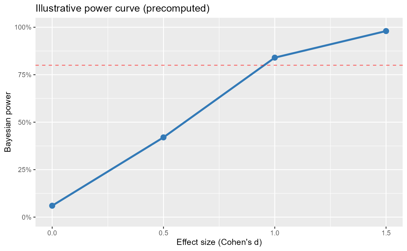

Interpreting the output

run_power_simulation() returns one row per effect size with these columns:

Column	Meaning
`effect_size`	Planned effect size (the value passed in `effect_sizes`)
`true_beta`	That effect size on the coefficient scale (baseline-SD units for standardized Gaussian)
`power`	Proportion of simulations satisfying the decision rule; the false-positive rate when `effect_size = 0`
`mc_se`	Monte Carlo standard error of `power`
`type_s`	Sign-error rate among simulations that fired
`type_m`	Average ratio of estimated to true magnitude among those that fired (exaggeration when above 1)
`n_valid`	Converged simulations used
`n_nonconverged`	Simulations dropped for Rhat > 1.01
`n_sims`	Simulations requested per effect size

effect_size = 0: estimates the false-positive rate; expect roughly 1 - prob_threshold (about 0.025 at the default 0.975).
Power >= 0.80: conventional adequacy threshold; 0.90 or 0.95 when stakes are higher.
More cases and time points per phase raise power.
Higher autocorrelation lowers effective sample size, lowering power.
Higher ICC (between-case heterogeneity) inflates standard errors, lowering power.

Decision rules

A simulation “fires” when its posterior meets the chosen rule. The three rules match the quantities the analysis functions report (pd, prob_meaningful_change, rope_prob): one asks about direction, two ask whether the effect is large enough to matter.

`decision_rule`	Fires when	Detail
`"prob_direction"`	The probability of direction reaches `prob_threshold` (default 0.975)	`max(P(beta > 0), P(beta < 0)) >= prob_threshold`
`"prob_meaningful"`	The posterior probability of an effect beyond the ROPE reaches `prob_threshold`	`max(P(beta >= rope), P(beta <= -rope)) >= prob_threshold`
`"rope"`	The posterior mass inside the ROPE drops below `1 - prob_threshold`	Nearly all mass falls outside `[-rope, +rope]`; the strictest rule

Coefficients

`coefficient`	Tests	When to use
`"level"`	Immediate phase-shift effect	Most SCED applications
`"trend"`	Baseline time trend	Pre-existing trend modeling
`"slope_change"`	Post-intervention slope change	Gradual treatment effects

Design + family combinations

Build the parameter grid first:

designs  <- c("ab", "reversal", "multiple_baseline")
families <- c("gaussian", "poisson", "negbinomial")
grid <- expand.grid(design = designs, family = families,
                    stringsAsFactors = FALSE)
grid
#>              design      family
#> 1                ab    gaussian
#> 2          reversal    gaussian
#> 3 multiple_baseline    gaussian
#> 4                ab     poisson
#> 5          reversal     poisson
#> 6 multiple_baseline     poisson
#> 7                ab negbinomial
#> 8          reversal negbinomial
#> 9 multiple_baseline negbinomial

Then iterate run_power_simulation() across rows interactively.

Single-subject mode

Set n_cases = 1 to fit without random effects (single-case piecewise regression). Power is based on within-subject variability only:

if (interactive()) {
  run_power_simulation(
    n_sims = 50, n_cases = 1,
    n_phase_a = 10, n_phase_b = 10,
    effect_sizes = c(0, 0.8, 1.5, 2.0),
    design = "ab", family = "gaussian"
  )
}

Runtime expectations

Scenario	Approx wall time
50 sims x 4 effect sizes, Gaussian, default iter/chains	10-20 min
100 sims x 6 effect sizes, Poisson/NB	30-60 min
50 sims x 4 effect sizes, n_cases = 1 (no random effects)	5-10 min

First runs include Stan compilation (~30-60 s per distinct model form); later runs reuse the cached model.

For larger jobs, use future::plan(future::multisession, workers = N) and parallelize across effect sizes manually.