suppressPackageStartupMessages({
  library(tidyverse)
  library(knitr)
  library(readxl)
  library(data.table)
  library(broom.mixed)
  library(DT)
  library(bibliometrix)
  library(openxlsx)
  library(sf)
  library(rnaturalearth)
  library(ggrepel)
  library(ggiraph)
  library(stringi)
  library(brms)
  library(performance)
  library(visNetwork)
  library(htmltools)
  library(RColorBrewer)
  library(flextable)
})

load("evolution/bayes_model.RData")Exploring the Research Landscape on Single-Case Design Methodology Using Technology Through Text Mining and Large Language Models
This website contains Data and R and Python code used for the analyses in Shin and McKenna (in press). The scripts were also posted through an online data repository at Center for Open Science and GitHub.
Shin, M., & McKenna, J. (in press). Exploring the research landscape on single-case design methodology using technology through text mining and large language models. Journal of Behavioral Education.
Pipeline
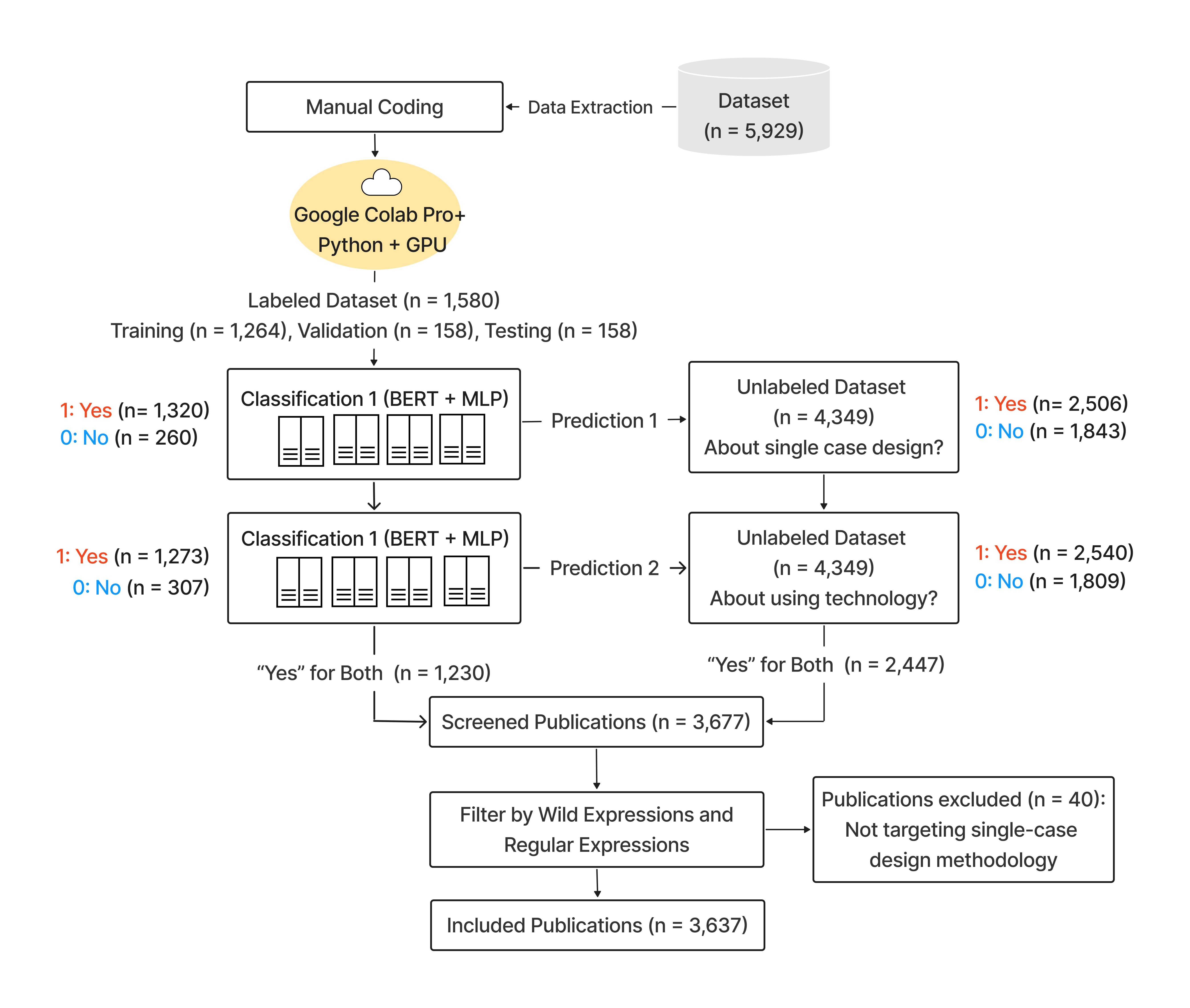
Semi-Automated Publication Screening
Search Strategy
Web of Science (All Fields): Single-case design (18 terms) AND technology terms (49 terms)
Setup Environment
Extract Web of Science (WoS) Data
wos_1_500 <- convert2df("1_500.ciw", dbsource = "wos", format = "endnote")
wos_501_1000 <- convert2df("501_1000.ciw", dbsource = "wos", format = "endnote")
wos_1001_1500 <- convert2df("1001_1500.ciw", dbsource = "wos", format = "endnote")
wos_1501_2000 <- convert2df("1501_2000.ciw", dbsource = "wos", format = "endnote")
wos_2001_2500 <- convert2df("2001_2500.ciw", dbsource = "wos", format = "endnote")
wos_2501_3000 <- convert2df("2501_3000.ciw", dbsource = "wos", format = "endnote")
wos_3001_3500 <- convert2df("3001_3500.ciw", dbsource = "wos", format = "endnote")
wos_3501_4000 <- convert2df("3501_4000.ciw", dbsource = "wos", format = "endnote")
wos_4001_4500 <- convert2df("4001_4500.ciw", dbsource = "wos", format = "endnote")
wos_4501_5000 <- convert2df("4501_5000.ciw", dbsource = "wos", format = "endnote")
wos_5001_5500 <- convert2df("5001_5500.ciw", dbsource = "wos", format = "endnote")
wos_5501_5935 <- convert2df("5501_5935.ciw", dbsource = "wos", format = "endnote")
Code
wos_5935 <- bind_rows(wos_1_500,
wos_501_1000,
wos_1001_1500,
wos_1501_2000,
wos_2001_2500,
wos_2501_3000,
wos_3001_3500,
wos_3501_4000,
wos_4001_4500,
wos_4501_5000,
wos_5001_5500,
wos_5501_5935)
wos <- wos_5935 %>%
filter(PY >= 1970)
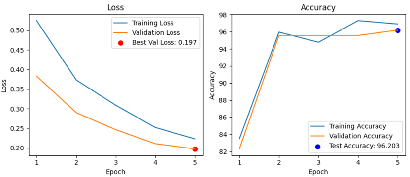
write.csv(wos, "init_all_data.csv", row.names = FALSE)Model Training and Validation for Document Classification Tasks
A Transformer-MLP classifier (pubmlp) combined transformer embeddings with categorical and numeric features for binary classification. The model was trained on human-labeled records and used to predict labels for unlabeled records. Classification was performed sequentially: first for single-case design, then for technology use.
Step 1. Text classification for single-case design
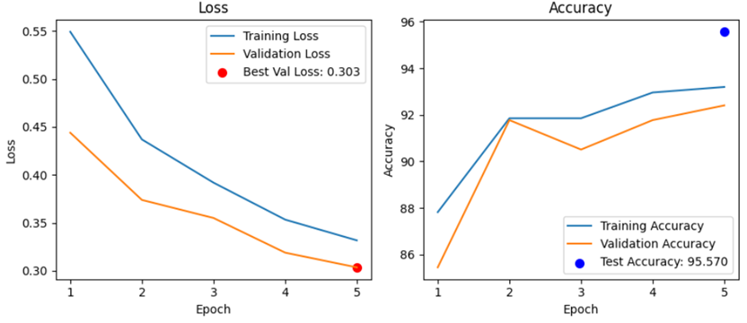
Step 2. Text classification for technology use
Step 3. Filtering studies including methodology content
Employed a list of 77 wildcard expressions using regular expressions to filter methodology content. See Code for the full list.
Descriptive Bibliometric Analysis
Main Findings
Code
data <- read.xlsx("../data/df.xlsx")

data <- data %>% filter(filtered == "Yes")

data_descriptive <- data %>%
  dplyr::mutate(Study = paste("study", row_number(), sep = "")) %>%
  dplyr::mutate(document = paste(Study, PY, sep = "_")) %>%
  ungroup()

data_descriptive <- data_descriptive %>%
  dplyr::select(document, everything())

data_descriptive$DT <- case_when(
  data_descriptive$DT == "ARTICLE" ~ "Article",
  data_descriptive$DT == "BOOK CHAPTER" ~ "Book Chapter",
  data_descriptive$DT == "ARTICLE; BOOK CHAPTER" ~ "Book Chapter",
  data_descriptive$DT == "REVIEW; BOOK CHAPTER" ~ "Book Chapter",
  data_descriptive$DT == "ARTICLE; DATA PAPER" ~ "Article",
  data_descriptive$DT == "EARLY ACCESS" ~ "Early Access",
  data_descriptive$DT == "ARTICLE; EARLY ACCESS" ~ "Article",
  data_descriptive$DT == "REVIEW; EARLY ACCESS" ~ "Review",
  data_descriptive$DT == "PROCEEDINGS PAPER" ~ "Proceeding Paper",
  data_descriptive$DT == "ARTICLE; PROCEEDINGS PAPER" ~ "Article",
  data_descriptive$DT == "REVIEW" ~ "Review",
  data_descriptive$DT == "EDITORIAL MATERIAL" ~ "Editorial Material",
  data_descriptive$DT == "MEETING ABSTRACT" ~ "Meeting Abstract",
  TRUE ~ as.character(data_descriptive$DT)
)

source_hindex <- bibliometrix::Hindex(data_descriptive, years = Inf, field = "source")$H
source_hindex$SO <- source_hindex$Element
source_hindex$m_index <- round(source_hindex$m_index, 2)

source_TC <- data_descriptive %>%
  dplyr::group_by(SO) %>%
  dplyr::summarize(total_citation = sum(TC)) %>%
  dplyr::mutate(total_citation_percent = round((total_citation / sum(total_citation) * 100),2)) %>%
  ungroup()

source_TP <- data_descriptive %>%
  dplyr::group_by(SO) %>%
  dplyr::summarize(publication_number = n()) %>%
  dplyr::mutate(publication_number_percent = round((publication_number / sum(publication_number) * 100),2)) %>%
  ungroup()

source_detail <- left_join(source_TC, source_TP, by = "SO")

source_detail <- source_detail %>%
  group_by(SO) %>%
  dplyr::mutate(citation_per_publication = round((total_citation / publication_number),0))

source_detail <- source_detail %>% arrange(desc(total_citation), desc(publication_number))
source_combined <- left_join(source_detail, source_hindex, by = "SO")
source_combined <- source_combined %>%
  arrange(desc(total_citation), desc(publication_number)) %>%
  select(SO, PY_start, publication_number, publication_number_percent,
         total_citation, total_citation_percent,
         citation_per_publication,
         h_index, g_index, m_index)


write.xlsx(source_combined, file = "files/source_combined.xlsx", colNames = TRUE)

results <- biblioAnalysis(data_descriptive)
descriptive_summary <- summary(results, k=71, pause=F, width=130)
MainInformationDF <- descriptive_summary$MainInformationDF

write.xlsx(MainInformationDF, file = "files/MainInformationDF.xlsx", colNames = TRUE)

MostProdCountries <- descriptive_summary$MostProdCountries

write.xlsx(MostProdCountries, file = "files/MostProdCountries.xlsx", colNames = TRUE)

TCperCountries <- descriptive_summary$TCperCountries

write.xlsx(TCperCountries, file = "files/TCperCountries.xlsx", colNames = TRUE)
Map Publications and Citations Across Countries
Code
MostProdCountries <- MostProdCountries %>%
  mutate(
    Articles = as.numeric(Articles),
    Freq = as.numeric(Freq),
    SCP = as.numeric(SCP),
    MCP = as.numeric(MCP),
    MCP_Ratio = as.numeric(MCP_Ratio)
  )

TCperCountries <- TCperCountries %>%
  mutate(
    `Total Citations` = as.numeric(`Total Citations`),
    `Average Article Citations` = as.numeric(`Average Article Citations`)
  )

colnames(TCperCountries) <- stringr::str_trim(colnames(TCperCountries))

Countries_Prod_TC <- MostProdCountries %>%
  left_join(TCperCountries, by = "Country")

Countries_Prod_TC <- Countries_Prod_TC %>%
  mutate(Country = str_trim(Country, "both") %>% str_to_title())

Countries_Prod_TC <- Countries_Prod_TC %>%
  mutate(Country = case_when(
    Country == "Usa" ~ "USA",
    Country == "Korea" ~ "South Korea",
    Country == "U Arab Emirates" ~ "UAE",
    Country == "United Kingdom" ~ "UK",
    TRUE ~ as.character(Country)
  ))

write.xlsx(Countries_Prod_TC, file = "files/Countries_Prod_TC.xlsx", colNames = TRUE)

sf::sf_use_s2(TRUE)

world <- ne_countries(scale = "small", returnclass = "sf")

world <- world %>%
  mutate(admin = case_when(
    admin == "United States of America" ~ "USA",
    admin == "United Arab Emirates" ~ "UAE",
    admin == "United Kingdom" ~ "UK",
    admin == "United Republic of Tanzania" ~ "Tanzania",
    admin == "Republic of Serbia" ~ "Serbia",
    TRUE ~ as.character(admin)
  ))

wintr_proj <- "+proj=wintri +datum=WGS84 +no_defs +over"

if (is.na(st_crs(world))) {
  st_crs(world) <- 4326
}

world_projected <- lwgeom::st_transform_proj(world, crs = wintr_proj)
centroids_projected <- st_centroid(st_geometry(world_projected))
centroids_geo <- st_transform(centroids_projected, crs = st_crs(world))
world_centroids <- cbind(world, st_coordinates(centroids_geo))
world_joined <- left_join(world, Countries_Prod_TC, by = c("admin" = "Country"))
world_joined_filtered <- world_joined %>% filter(!is.na(Articles))
world_joined_filtered <- world_joined_filtered %>%
  mutate(country_article = paste(admin, Articles))

world_sf <- st_as_sf(world_joined_filtered, coords = c("longitude", "latitude"), crs = "+proj=longlat +datum=WGS84 +ellps=WGS84 +towgs84=0,0,0")

b <- c(200, 2000, 5000, 10000, 20000, 40000, 60000, 70000)

world_map_init <- world_sf %>%
  ggplot() +
  geom_sf_interactive(aes(fill = `Total Citations`,
                          tooltip = paste("TC: ", admin, `Total Citations`)),
                      size = 0.25) +
  geom_label_repel(
    size = 3.3,
    aes(geometry = geometry, label = admin),
    alpha = 0.7,
    max.overlaps = 13,
    stat = "sf_coordinates"
  ) +
  scale_fill_viridis_c(trans = "sqrt", na.value = "white", breaks = b, direction = -1, alpha = 0.9, begin = 0.6, end = 1) +
  geom_point_interactive(
    aes(size = Articles,
        geometry = geometry,
        tooltip = paste("TP: ", admin, Articles)),
    stat = "sf_coordinates",
    stroke = 1,
    shape = 21,
    color = "#A84268",
    alpha = 0.6
  ) +
  theme_void() +
  theme(
    legend.position = "bottom",
    legend.direction = "horizontal",
    legend.title = element_text(size = 11),
    legend.text = element_text(size = 10)
  ) +
  labs(fill = "Total citations (TC)", size = "Total publications (TP)") +
  guides(
    fill = guide_colourbar(title.position = "top", title.hjust = 0.5, barwidth = 18, barheight = 1),
    size = guide_legend(title.position = "top", title.hjust = 0.5)
  )

world_map <- girafe(ggobj = world_map_init, width_svg = 10, height_svg = 5) %>%
  girafe_options(
    opts_hover(css = "fill:cyan;"),
    opts_sizing(rescale = TRUE),
    css = "div.girafe-container { padding-top: 0px; margin-top: -20px; }
           .ggiraph-toolbar { position: absolute; bottom: 10px; right: 10px; }"
  )

htmlwidgets::saveWidget(
  widget = world_map,
  file = "world_map/index.html",
  selfcontained = TRUE)

ggsave('files/world_map.png',
       width = 7, height = 3.5, dpi = 300, plot = world_map_init)

save(world_map, file = "files/world_map.RData")
Figure 3. Map of Publications and Citations Across Countries
Contextualized Topic Modeling and LLM-Assisted Topic Labeling
Word Co-Occurrence Network Analysis
Interactive Word Networks
Word Usage Summary
Code
message("\nGenerating word usage summary...")
df_summary <- read_excel("../data/df.xlsx", col_types = "text") %>%
mutate(
Year = as.numeric(Year),
across(c(Topic, CustomLabel, unigrams, bigrams, trigrams), as.character)
)
extract_ngrams <- function(data, type) {
data %>%
select(UT, WC, Year, Topic, tokens = all_of(type)) %>%
filter(!is.na(tokens), !tokens %in% c("", "[]", "['']", '[""]')) %>%
mutate(
tokens = str_replace_all(tokens, "^\\[|\\]$", ""),
tokens = str_replace_all(tokens, "^'|'$", ""),
tokens = str_replace_all(tokens, '^"|"$', ""),
tokens = str_replace_all(tokens, "\\'", ""),
tokens = str_replace_all(tokens, '\\"', ""),
tokens = str_split(tokens, ",\\s*")
) %>%
unnest(tokens) %>%
filter(tokens != "", !is.na(tokens)) %>%
mutate(
tokens = str_trim(tokens),
tokens = str_replace_all(tokens, "^'|'$", ""),
tokens = str_replace_all(tokens, '^"|"$', ""),
tokens = str_replace_all(tokens, "\\'", ""),
tokens = str_replace_all(tokens, '\\"', "")
) %>%
filter(tokens != "", !is.na(tokens)) %>%
rename(ngram = tokens) %>%
mutate(
ngram_type = type,
ngram = str_trim(ngram)
)
}
ngram_types <- c("unigrams", "bigrams", "trigrams")
available <- intersect(ngram_types, names(df_summary))
ngrams_concat <- map_dfr(available, ~ extract_ngrams(df_summary, .x))
unigrams_df <- ngrams_concat %>%
filter(ngram_type == "unigrams") %>%
mutate(
Decade = paste0(floor(Year/10)*10, "s")
)
first_year <- unigrams_df %>%
group_by(ngram) %>%
summarize(Year0 = min(Year, na.rm = TRUE), .groups = "drop") %>%
mutate(FirstDecade = paste0(floor(Year0/10)*10, "s"))
unigrams_df <- unigrams_df %>%
left_join(first_year %>% select(ngram, FirstDecade), by = "ngram")
write.xlsx(unigrams_df, "evolution/unigrams_df.xlsx", rowNames = FALSE)
process_tokens <- function(tokens) {
tokens_clean <- tokens[!is.na(tokens)]
tokens_clean <- str_trim(tokens_clean)
tokens_clean <- tokens_clean[tokens_clean != ""]
if (length(tokens_clean) == 0) {
return(tibble::tibble(
Total_Word_Count = 0L,
Min = NA_integer_,
Q1 = NA_real_,
Median = NA_real_,
Mean = NA_real_,
Q3 = NA_real_,
Max = NA_integer_,
Skew = NA_real_,
Kurt = NA_real_,
Distinct_Word_Count = 0L,
Count_Once = 0L,
Count_More_Than_Once = 0L
))
}
freq <- as.integer(table(tokens_clean))
skew_val <- if (length(freq) > 1 && var(freq) > 0) round(moments::skewness(freq), 2) else NA_real_
kurt_val <- if (length(freq) > 1 && var(freq) > 0) round(moments::kurtosis(freq), 2) else NA_real_
tibble::tibble(
Total_Word_Count = sum(freq),
Mean = round(mean(freq), 2),
SD = round(sd(freq), 2),
Min = min(freq),
`25th pct` = as.numeric(quantile(freq, .25)),
`50th pct` = median(freq),
`75th pct` = as.numeric(quantile(freq, .75)),
Max = max(freq),
Skew = skew_val,
Kurt = kurt_val
# Distinct_Word_Count = length(freq),
# Count_Once = sum(freq == 1L),
# Count_More_Than_Once = sum(freq > 1L)
)
}
decades <- unigrams_df %>%
pull(Decade) %>%
unique() %>%
na.omit() %>%
sort()
decade_stats <- purrr::map_dfr(decades, function(d) {
sub <- dplyr::filter(unigrams_df, Decade == d)
stats <- process_tokens(sub$ngram)
topic_stats <- sub %>%
group_by(Topic) %>%
summarise(
topic_word_count = n(),
topic_new_words = sum(FirstDecade == d),
topic_reused_words = sum(FirstDecade < d),
.groups = "drop"
)
reused <- sub %>%
filter(!is.na(FirstDecade) & FirstDecade < d) %>%
pull(ngram)
reused_tab <- sort(table(reused), decreasing = TRUE)
new <- sub %>%
filter(FirstDecade == d) %>%
pull(ngram)
new_tab <- sort(table(new), decreasing = TRUE)
stats %>%
mutate(
Decade = d,
`All words` = Total_Word_Count,
`Reused words` = sum(reused_tab),
`New words` = sum(new_tab),
Topic = nrow(topic_stats),
`Top 10 reused words` = if (length(reused_tab))
paste(names(head(reused_tab, 10)), collapse = ", ")
else
NA_character_,
`Top 10 new words` = if (length(new_tab))
paste(names(head(new_tab, 10)), collapse = ", ")
else
NA_character_
) %>%
select(
Decade,
`All words`,
`Reused words`,
`New words`,
Topic,
`Top 10 reused words`,
`Top 10 new words`,
Mean,
SD,
Min,
`25th pct`,
`50th pct`,
`75th pct`,
Max,
Skew,
Kurt
# Distinct_Word_Count,
# Count_Once,
# Count_More_Than_Once
)
})
topic_decade_stats <- unigrams_df %>%
group_by(Topic, Decade) %>%
summarise(
Word_Count = n(),
New_Words = sum(FirstDecade == Decade),
Reused_Words = sum(FirstDecade < Decade),
.groups = "drop"
) %>%
arrange(Topic, Decade)
word_usage_df <- decade_stats %>%
mutate(across(-Decade, as.character)) %>%
tidyr::pivot_longer(
cols = -Decade,
names_to = "Metric",
values_to = "Value"
) %>%
tidyr::pivot_wider(
names_from = Decade,
values_from = Value
)
openxlsx::write.xlsx(
list(
"Decade_Summary" = word_usage_df,
"Topic_Decade_Summary" = topic_decade_stats
),
"evolution/word_usage_summary.xlsx"
)
word_usage_table <- DT::datatable(
word_usage_df,
options = list(
dom = 'Bfrtip',
buttons = c('copy', 'csv', 'excel', 'pdf'),
pageLength = 10,
scrollX = TRUE
),
extensions = 'Buttons',
class = "cell-border stripe",
rownames = FALSE
)
count_new_word_topic_year <- function(df) {
df %>%
group_by(Topic, Year) %>%
summarise(ngram = list(unique(ngram)), .groups = "drop") %>%
arrange(Topic, Year) %>%
group_by(Topic) %>%
mutate(
cum_union = purrr::accumulate(ngram, union),
previous_words = dplyr::lag(cum_union, default = list(character(0))),
new_words = purrr::map2(ngram, previous_words, setdiff),
Count = purrr::map_int(new_words, length)
) %>%
select(Topic, Year, Count)
}
new_word_count_df <- count_new_word_topic_year(unigrams_df)
topic_levels <- unique(new_word_count_df$Topic)
topic_levels <- topic_levels[order(as.numeric(topic_levels))]
new_word_count_df$Topic <- factor(new_word_count_df$Topic, levels = topic_levels)
new_word_count_df$Decade <- paste0(floor(new_word_count_df$Year/10)*10, "s")
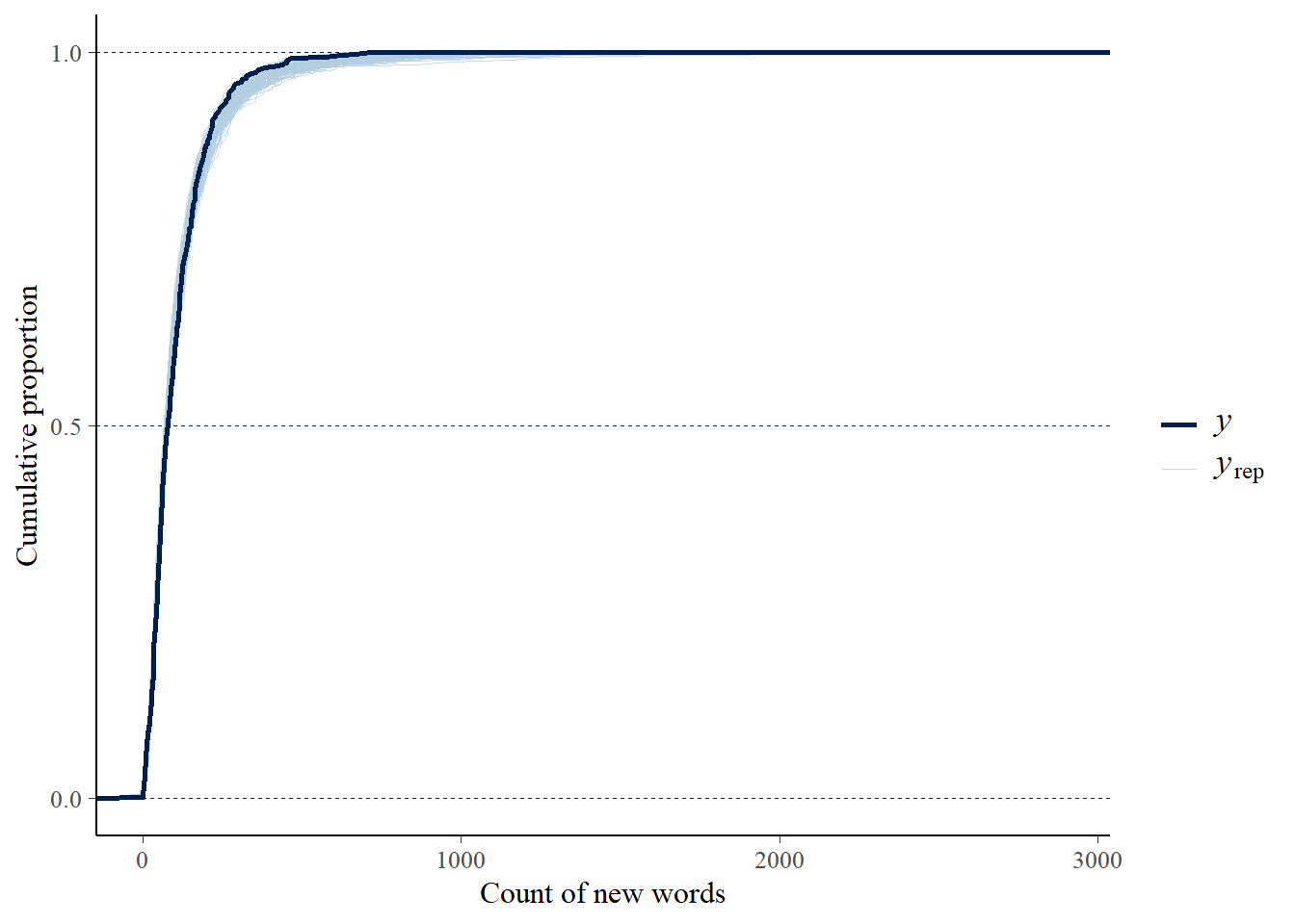
write.xlsx(new_word_count_df, file = "evolution/new_word_count_df.xlsx", colNames = TRUE)Bayesian Negative Binomial Piecewise Regression
Dispersion Ratio
Code
mean_val <- mean(new_word_count_df$Count)
var_val  <- var(new_word_count_df$Count)
overdispersion_ratio <- var_val / mean_val
overdispersion_ratio
[1] 87.501Preprocess
new_word_count_data <- new_word_count_df %>%
  group_by(Topic) %>%
  mutate(
    year_c = Year - min(Year, na.rm = TRUE),
    post_2010 = as.integer(Year >= 2010),
    post_2010_years = (Year - 2010) * post_2010
  ) %>%
  ungroup()
Estimate the Model
Code
new_word_count_data$Topic <- as.factor(new_word_count_data$Topic)
new_word_count_data$Topic <- relevel(new_word_count_data$Topic, ref = "4")

formula_new_word <- bf(
  Count ~ 1 + year_c + post_2010 + post_2010_years +
    Topic + year_c:Topic + post_2010:Topic + post_2010_years:Topic
)

priors_new_word <- c(
  prior(normal(0, 5), class = "Intercept"),
  prior(normal(0, 2), class = "b")
)

model_new_word <- brm(
  formula = formula_new_word,
  data = new_word_count_data,
  family = negbinomial(link = "log"),
  prior = priors_new_word,
  control = list(adapt_delta = 0.95, max_treedepth = 12),
  iter = 2000,
  warmup = 1000,
  cores = 4,
  chains = 4,
  seed = 2025
)

coefs <- fixef(model_new_word)

topic_labels_df <- readxl::read_excel("../data/df.xlsx", col_types = "text") %>%
  select(Topic, CustomLabel) %>%
  distinct()

topic_starts <- new_word_count_df %>%
  group_by(Topic) %>%
summarise(First_Year = as.character(min(Year, na.rm = TRUE)), .groups = "drop")Posterior Predictive Checks
Piecewise Contrasts Between Topics
Code
topics <- sort(as.integer(str_extract(
  grep("^Topic\\d+$", rownames(coefs), value = TRUE), "\\d+"
)))
var_order <- c("Intercept", "year_c", "post_2010", "post_2010_years",
  paste0(rep(c("", "year_c:", "post_2010:", "post_2010_years:"), times = length(topics)),
         "Topic", rep(topics, each = 4)))

model_new_word_results <- coefs %>%
  as.data.frame() %>%
  tibble::rownames_to_column("Variable") %>%
  mutate(
    IRR = exp(Estimate),
    IRR_Q2.5 = exp(Q2.5),
    IRR_Q97.5 = exp(Q97.5),
    across(where(is.numeric), ~round(., 2)),
    Variable = factor(Variable, levels = var_order)
  ) %>%
  arrange(Variable) %>%
  mutate(Variable = as.character(Variable))

model_new_word_results_apa <- model_new_word_results %>%
  mutate(
    `Est (SD)` = sprintf("%.2f (%.2f)", Estimate, Est.Error),
    `95% CI` = sprintf("[%.2f, %.2f]", Q2.5, Q97.5),
    `IRR` = sprintf("%.2f", IRR),
    `IRR 95% CI` = sprintf("[%.2f, %.2f]", IRR_Q2.5, IRR_Q97.5),
    Sig = ifelse(Q2.5 > 0 | Q97.5 < 0, "*", "")
  ) %>%
  select(Variable, `Est (SD)`, `95% CI`, IRR, `IRR 95% CI`, Sig)

save_as_docx(flextable(model_new_word_results_apa),
             path = "evolution/model_new_word_results_apa.docx")
Piecewise Regressions by Topic
Code
topics_other <- setdiff(levels(new_word_count_data$Topic), "4")
effects <- c("Intercept", "year_c", "post_2010", "post_2010_years")

hyp_strings <- c(
  # Topic 4 (reference) — main effects are the total effects
  "Intercept = 0",
  "year_c = 0",
  "post_2010 = 0",
  "post_2010_years = 0",
  # Other topics — main + interaction = total effect
  paste0("Intercept + Topic", topics_other, " = 0"),
  paste0("year_c + year_c:Topic", topics_other, " = 0"),
  paste0("post_2010 + post_2010:Topic", topics_other, " = 0"),
  paste0("post_2010_years + post_2010_years:Topic", topics_other, " = 0")
)

hyp <- hypothesis(model_new_word, hyp_strings)

n_other <- length(topics_other)
topic_vec <- c(rep("4", 4), rep(topics_other, 4))
effect_vec <- c(effects, rep(effects, each = n_other))

per_topic_effects <- hyp$hypothesis %>%
  mutate(
    Topic = topic_vec,
    Variable = effect_vec,
    IRR = exp(Estimate),
    IRR_lower = exp(CI.Lower),
    IRR_upper = exp(CI.Upper),
    Sig = ifelse(CI.Lower > 0 | CI.Upper < 0, "*", "")
  ) %>%
  left_join(topic_labels_df, by = "Topic") %>%
  left_join(topic_starts, by = "Topic") %>%
  mutate(
    `Topic` = paste0(Topic, ": ", CustomLabel),
    `Est (SD)` = sprintf("%.2f (%.2f)", Estimate, Est.Error),
    `95% CI` = sprintf("[%.2f, %.2f]", CI.Lower, CI.Upper),
    `IRR` = sprintf("%.2f", IRR),
    `IRR 95% CI` = sprintf("[%.2f, %.2f]", IRR_lower, IRR_upper)
  ) %>%
  select(Topic, First_Year, Variable, `Est (SD)`, `95% CI`, IRR, `IRR 95% CI`, Sig) %>%
  arrange(as.integer(str_extract(Topic, "^\\d+")), factor(Variable, levels = effects))

save_as_docx(flextable(per_topic_effects),
             path = "evolution/per_topic_effects.docx")
Predicted New Word Trajectories
Code
predData <- expand.grid(
  Year = seq(min(new_word_count_df$Year), max(new_word_count_df$Year), by = 1),
  Topic = unique(new_word_count_df$Topic)
)

predData <- predData %>%
  left_join(topic_starts %>% mutate(First_Year = as.integer(First_Year)), by = "Topic") %>%
  mutate(
    year_c = Year - First_Year,
    post_2010 = as.integer(Year >= 2010),
    post_2010_years = (Year - 2010) * post_2010
  ) %>%
  select(-First_Year)

pred <- predict(model_new_word, newdata = predData, probs = c(0.025, 0.975))
predData$pred <- pred[, "Estimate"]
predData$lower <- pred[, "Q2.5"]
predData$upper <- pred[, "Q97.5"]

new_word_gg <- ggplot() +
  geom_point(data = new_word_count_df,
             aes(x = Year, y = Count, group = Topic),
             size = 1, alpha = 0.4) +
  geom_line(data = predData,
            aes(x = Year, y = pred, group = Topic),
            color = "blue", linewidth = 0.5, alpha = 0.7) +
  geom_ribbon(data = predData,
              aes(x = Year, ymin = lower, ymax = upper, group = Topic),
              fill = "blue", alpha = 0.1) +
  labs(
    x = "Year",
    y = "New Word Count"
  ) +
  facet_wrap(~ Topic, ncol = 3, scales = "free_y",
             labeller = labeller(Topic = function(x) paste("Topic", x))) +
  scale_x_continuous(
    breaks = seq(1970, 2020, by = 20),
    limits = c(1970, 2025),
    expand = expansion(0, 0)
  ) +
  theme_minimal(base_size = 12) +
  theme(
    panel.grid.minor   = element_blank(),
    panel.grid.major.x = element_line(color = "gray90"),
    panel.grid.major.y = element_line(color = "gray90"),
    strip.text         = element_text(size = 12),
    axis.line.x        = element_line(color = "gray90"),
    axis.line.y        = element_line(color = "gray90"),
    axis.ticks.length  = unit(0.2, "cm"),
    axis.text.x        = element_text(size = 12),
    axis.text.y        = element_text(size = 12),
    axis.title.x       = element_text(
      size   = 12,
      margin = margin(t = 5)
    ),
    axis.title.y       = element_text(
      size   = 12,
      margin = margin(r = 12),
      angle  = 90,
      vjust  = 0.5
    ),
    plot.title = element_text(face = "bold", hjust = 0.5),
    plot.subtitle = element_text(hjust = 0.5, color = "gray40"),
    plot.caption = element_text(size = 10, color = "gray40"),
    legend.position = "bottom"
  )